Keywords: Kernel estimators, Parzen method, indirect observations, uncertain data, regularization, deconvolution, Lucy?s distribution rectification.
The estimation of probability density functions form random samples is a basic problem in several domains of applied sciences, machine learning among them. In many situations, samples are not directily known: they may have suffered some random perturbations in the form of noise in the measurement process, or, simply, they are subjective judgements about the true values. Our paper addresses the problem of estimating a probability density function p(x), given a random sample of size n of indirect observations, modeled by n likelihoods functions {li(xi) º p(si|xi)}. Each of them describes the statistical properties of the "measurement process" of each sample: si is the available observed magnitude, related to the true sample xi .
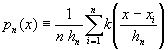
Kernel method is the non-parametric technique used in our approach to density estimation, but conveniently adapted to cope with uncertainty in the observations. In this method, also known as Parzen density estimation, a function p(x) from a sample {xi} is approximated with the following empirical density:
where k(x) is usually a smooth density function called the kernel function. Parzen?s method with normal kernels can be obtained by Tikhonov?s Regularization method for solving ill-posed problems, using the norm of the density as stabilizer functional.
For our purposes of managing uncertainty, we can justify Parzen method as follows: Given a probability density function p(x), a smooth version b(x) can be obtained by convolution with a kernel kh(x). Clearly, if the window width h is small enough, b(x) will be acceptably close to p(x). Additionally, the convolution with a probability density function can be empirically approximated over the random sample {xi}:
The fact that only a finite sample is available implies that the expected value must be changed to an empirical average. This necessarily requires some kind of regularization process, which in this case is achieved by using positive width (smoothing) kernel, instead of Dirac impulses, located at the samples.
Kernel Density Estimation from Indirect Measurements
Let p(x) be the probability density function to be estimated. The samples xi are not directly observed, and the only thing we have are the indirect measures si, related to the true values xi by the likelihoods functions li(xi). The density of the observable magnitude is related to the target density p(x) by:
From the fact that p(x) and q(s) are probability density functions, we can expand the solution p(x) in terms of q(s):
This way, we can see that the convolution operator q(s\x) (introduced by uncertainty in the observation process) has an "inverse" operator with a kernel that can be obtained from the basic conditional probability relations (Bayes theorem). Again, if we approximate an expected value by empirical average over the observations, we can obtain the following expression:
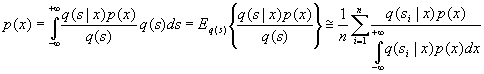
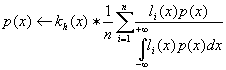
where, unfortunately, the expression for the inverse operator depends on the unknown density. But this formal manipulation suggest a general iterative technique to solve p(x): In each step, the expected value is approximated by empirical average over the observations, and then p(x) is updated from the estimation computed in the previous step. Additionally, as we said before, empirical approximation needs some kind of regularization, e.g. through convolution with a smoothing kernel (otherwise, exact observations would contribute to p(x) with weighted impulses). Therefore, the final update expression will be written as:
The EDR (Empirical Deconvolution by Regularization) Algorithm
In order to obtain a practical algorithm, we focus in the following reasonable situation:
a) The approximation for p(x) will have the following form:
where the "kernel" functions are no longer fixed width kernels located at fixed positions, but shifted versions with variable widths. The y i(x) functions can be computed as follows (being y i?(x) the elements of the summatory in the p(x) update expression given above):
b) The smoothing kernel is gaussian:
d) The components y? (and hence y) are approximated by gaussian densities:
This is a reasonable assumption since they are obtained as the result of a weighted sum of a large number of functions.
With this assumptions, we show how we can take advantage of the conjugate properties of the gaussian density, that allows analytic computation of the required products and integrals, avoiding numerical techniques. The essential term in the p(x) update expression becomes:
where
Now we define the following coefficients:
and the normalized weights:

in such a way that the components y? are given by:
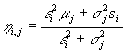
Therefore, the parameters of each component y?, approximated by gaussians, are updated by:
Finally, the parameters of the final (smoothed) components y = kh * y? are directly obtained from equation si2=s,i2+h2. The quality of kernel estimators can only be guaranteed asymptotically. In practical applications, the selection of the smoothing parameter h can be made using several techniques, including different values hi for each sample. We used several of these techniques in our experiments. In particular, cross-validation (based on the maximum pseudo leave-one-out likelihood) can be easily adapted to the method. Non parametric density estimation for finite sample sizes can also be derived from Vapnik?s Structural Risk Minimization principle. This approach will be studied in future works.
Starting from a first approximation to p(x) with mi=si and si=0, (which is equivalent to ignoring the amount of uncertainty in the observations) we iteratively update mi and si from the observations {(si, ei)}, until convergence. Experiments evidence that the algorithm attains the solution (a fixed point of the "inverse" operator) in a small number of steps (typically < 10).
An illustrative physical analogy can be loosely established between the EDR algorithm and a mechanical system composed by gravitational masses 1/s located at m, joined by elastic strips with strength 1/e to locations s. Masses attract to one another, but they cannot move too far due to the progressively increasing elastic force. The fixed point of the EDR iterative algorithm corresponds to the equilibrium point of this mechanical system.
Examples
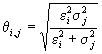
Finally, we give two figures that evidence the ability of the EDR algorithm to recover true densities through uncertatin observations. Figure 1 shows a one-dimensional case, in which an arbitrary non-parametric density is estimated through 400 inexact measures, perturbed with several noise values e i, uniformly distributed from 0 to 3. The darker line corresponds to the true density function, and the lighter to the EDR estimation, achieved in 12 iterations. Compare it with the p(x) estimated in the initial step (third line, dark gray), corresponding to a simple Parzen method, not taking into account the uncertainity, but only the centers of the inexact observations, si.
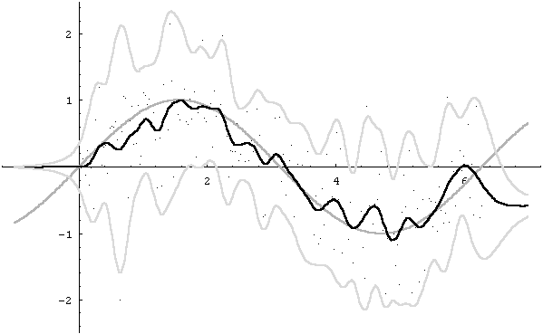
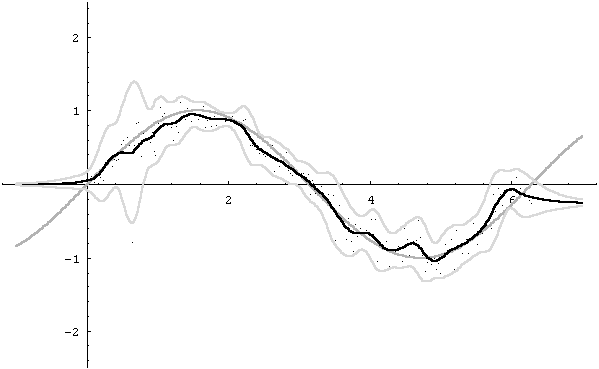
Figure 2, finally, shows, at the same time, how the algorithm is easily extended to manage multidimensional data (with factorized gaussian kernels), and how it can be used for non-parametric functional regression. We generated 200 equidistant X values in the interval [0,2p ], and, for each of these values, we calculated the corresponding Y value as the sin function of the X value, plus a gaussian noise with zero bias and deviations uniformly distributed in the [0,1] interval. Figure 2a shows the regression in the initial iteration (corresponding to ignoring uncertainity), and with points located at the center of the input observations. Figure 2b shows the final solution, obtained in 10 iterations, and where the points are located at the center of the "moved" kernels. Observe that the obtained regression curve (black) is a better approximation of the sin function (gray), and that the confidence interval, corresponding to ± 2 deviations, (light gray lines) is significantly narrower.
References